Collective Communications: The Operations Behind Every AI Network Flow

Part 3 of a series on data center networking for AI

Every distinctive traffic pattern discussed in this series, including the elephant flows, the synchronized barriers, the incast bursts, comes from a small, well-defined set of operations called collective communications. If Part 1 explained why AI traffic looks different, and Part 2 explained how a GPU physically reaches the network, this post explains exactly what that traffic is: the specific operations that move data between GPUs, and the network pattern each one produces.

These operations originate from MPI (Message Passing Interface) and are implemented for GPUs primarily through NCCL (NVIDIA’s collective communications library – pronounced “Nickel”). Every distributed training job and multi-GPU inference deployment is built from combinations of them.

First, let’s cover some basics

A neural network model is, physically, just a giant collection of numbers called parameters or weights. Think of them as the dials that get tuned during training. A large model might have billions of these numbers, organized into big grids called tensors (a tensor is just a generalization of a matrix, which could be 1-D, 2-D, or higher-dimensional array of numbers).

Here is a basic breakdown of a training loop:

1. Feed the model some data (a “batch” of examples)
2. The model makes a prediction (forward pass)
3. Compare the prediction to the correct answer. The gap is the “loss” (how wrong it was)
4. Figure out, for every single one of those billions of parameters, “which direction and how much should I nudge this number to make the loss smaller next time?” This per-parameter nudge value is a gradient
5. Apply the nudge to every parameter (update step)
6. Repeat, thousands to millions of times

Just to add to this, a gradient is simply: one number per parameter, telling you how to adjust that parameter to reduce error. If the model has 10 billion parameters, the gradient is a tensor of 10 billion numbers (one per weight).

Before we get into the collective operations themselves, two terms get used loosely and are worth defining, because they mean different things:

• Shard – a partition of something assigned permanently to a specific GPU as part of the overall job design. A data shard means GPU 3 permanently owns a slice of the training batch. A weight shard means GPU 3 permanently owns a slice of the model’s parameters. So when we hear “each GPU processes its own data shard,” it means: the training engineer split the full batch of data into pieces ahead of time, and GPU 3 permanently owns piece 3. When we hear “the weights are sharded across GPUs,” they mean the parameters themselves were split up and GPU 3 permanently owns a slice of the weight matrix. Sharding is about ownership, meaning which GPU is responsible for which piece, for the life of the whole job.
• Chunk – a temporary subdivision of a message, used purely to move data efficiently across the network. A multi-gigabyte gradient tensor gets sliced into smaller chunks so a collective operation can pipeline the transfer (start sending chunk 1 to the next GPU while still receiving chunk 2 from the previous one) rather than moving one giant blob in a single shot. Chunking is about how a transfer gets moved, not who owns what.

So, sharding is a design decision (made once, before the job runs). Chunking is a mechanical detail of how any given collective operation moves bytes efficiently (handled automatically by NCCL). Sharding is a durable, job-wide assignment; chunking is a transient, per-message wire mechanism.

The four foundational patterns

Every collective operation is a combination of four basic patterns: one-to-many, many-to-one, with or without a combining operator (sum, average, max). Recall, these come from MPI/NCCL, and every distributed training or multi-GPU inference job is built from combinations of them.

Broadcast – One GPU has data and sends an identical copy to every other GPU. As a network pattern, we can think of this as a one-to-many fan-out, with the same payload going to each destination, similar to a network broadcast.

Scatter – One GPU has a large buffer, splits it into distinct chunks, and sends a different chunk to each destination. As a network pattern, this is a one-to-many fan-out, but every destination receives different data.

Gather – This is the inverse of scatter where every GPU sends its chunk to one destination, which assembles them into a complete buffer. As a network pattern, this is a many-to-one incast, which I called out in Part 1 because network optimization mechanisms that avoid switch buffer exhaustion and packet drops are critical for handling this type of traffic pattern.

Reduce – Every GPU holds a value, and a combining operator (sum, max, average) merges them into a single result that lands on one destination GPU. As a network pattern, this is a many-to-one, with computation applied either en route or at the destination. In the diagram, three GPUs holding 3, 7, and 2 reduce to a single GPU holding 12. In an actual training job, each “value” is a tensor of billions of numbers (the gradient), and the reduce sums them element-by-element: position 1 of GPU0’s gradient adds to position 1 of GPU1’s gradient, and so on.

Now that we know what the 4 foundational patterns are, let’s go over the combined collective patterns in their own sections, including:

• All-reduce
• Reduce-scatter
• All-gather
• All-to-all

All-reduce: the workhorse of data-parallel training

First, what is data-parallel training? In simple terms, you have a model too slow to train on one GPU’s worth of data in reasonable time, so you make 4 identical copies of the full model, one per GPU. This is “data parallelism”. The model isn’t split, the data is.

In data-parallel training, every GPU holds an identical full copy of the model. The training batch is split into shards, one per GPU. GPU 0 sees examples 1-1000, GPU 1 sees 1001-2000, and so on. Each GPU independently runs forward + backward pass on its own data shard and computes a gradient, which is a tensor with one number per model parameter, describing how much and in which direction that parameter should be adjusted to reduce prediction error based on the data it saw.

Because each GPU saw different data, its gradient is different from every other GPU’s. If each GPU applied its own gradient independently, the model copies would drift apart and stop being identical, so you’d effectively have 4 different models, not one being trained faster. All-reduce solves this by summing (or averaging) all the gradient tensors together, element by element, and ensures every GPU receives the same combined result. Every GPU then applies an identical update, keeping all copies of the model in sync while still benefiting from having collectively seen far more data per step than any single GPU processed alone.

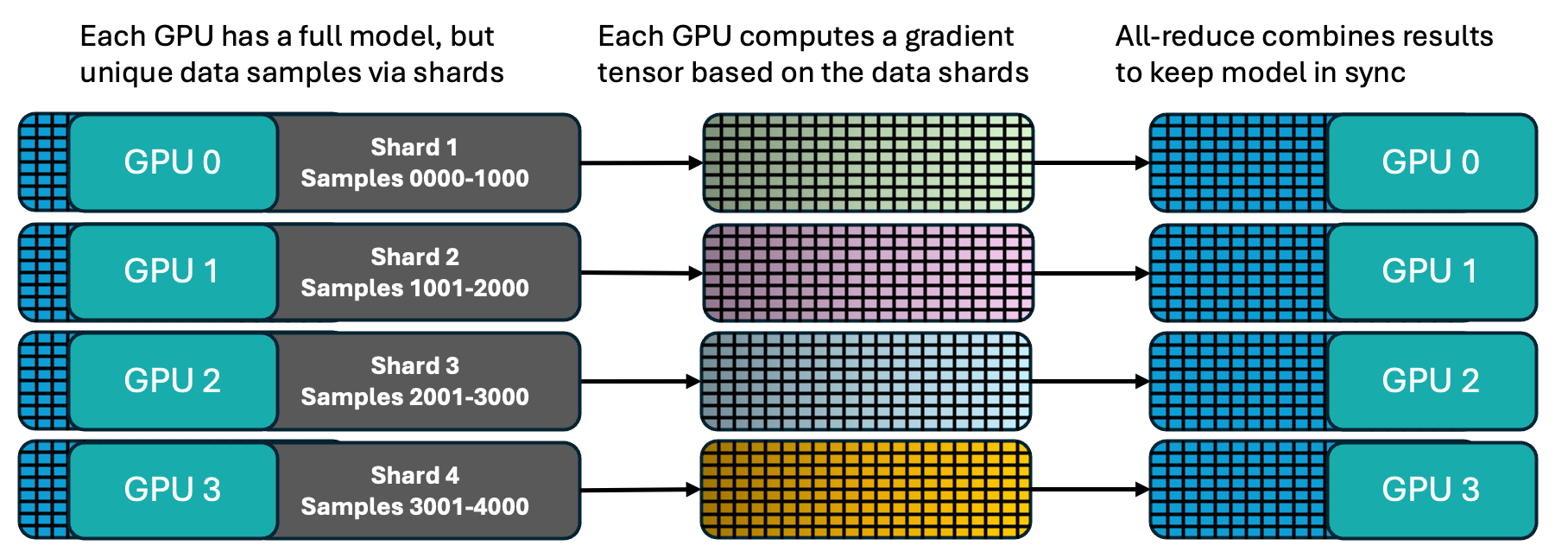
By default, NCCL uses a ring algorithm where GPUs are arranged in a logical ring, and the operation decomposes into two phases – reduce-scatter, then all-gather – with each GPU only ever talking to its two ring-neighbors. This keeps the algorithm bandwidth-optimal regardless of how many GPUs participate, and it’s topology-aware, meaning NCCL will construct the logical ring to match physically adjacent GPUs wherever possible, which is why the rail-optimized wiring from Part 2 matters.

The entire reason all-reduce exists is to let you train on many GPUs in parallel while keeping every copy of the model mathematically identical.

Reduce-scatter and all-gather: the two phases, visualized

Reduce-scatter combines reduce and scatter: the reduction happens, but instead of the combined result landing on one (or every) GPU, each GPU ends up holding only its own slice of the reduced result.

Walking through what this shows, with two GPUs and a gradient tensor split into two chunks (A and B):

• Start: both GPUs hold their own local, unreduced version of both chunks.
• After reduce-scatter: GPU 0 ends up holding only chunk A, but now fully summed across both GPUs. Its own copy of chunk B was sent away and combined into GPU 1’s copy instead. Neither GPU holds the complete tensor anymore; each holds only its assigned slice, already fully reduced.
• After all-gather: each GPU sends its completed slice to the other, so both end up holding the complete, fully-reduced tensor.

Now, why bother with the reduce-scatter step at all instead of just doing a full all-reduce that gives everyone everything? This is the FSDP (Fully Sharded Data Parallel) memory approach: if your parameters are also sharded (GPU0 permanently owns weight-slice A, GPU1 permanently owns weight-slice B), then GPU0 only ever needs the gradient for the weights it owns. It never needs to hold B’s gradient in memory at all. This is how you train models too large to fit on a single GPU. The idea is to avoid ever materializing the “whole thing” anywhere. Regular all-reduce (which gives everyone the full result) is simpler but wastes memory when you don’t need the full tensor everywhere, whereas reduce-scatter is the memory-frugal version.

All-gather and tensor parallelism: why this matters just as much for inference

All-gather is the inverse of scatter: each GPU holds a distinct chunk, and after the operation, every GPU holds the full, reassembled set. This is the second phase of ring all-reduce above, but it’s also, independently, one of the most important patterns for inference, which is where most enterprise AI workloads live.

Tensor parallelism takes a different approach than data parallelism. Instead of copying the whole model and splitting the data, it splits the model itself. A weight matrix is cut into slices, and each GPU is permanently assigned one slice.

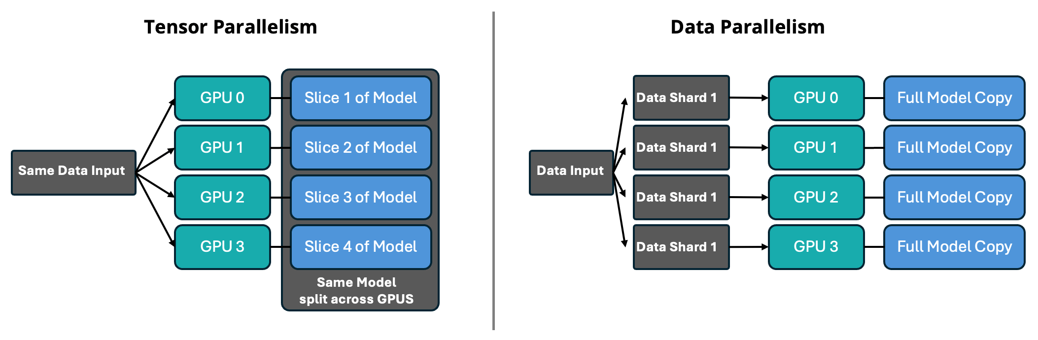
For example: if a layer’s output is 4096 numbers wide, four-way tensor parallelism might cut the weight matrix into four column-slices of 1024 each, one per GPU.

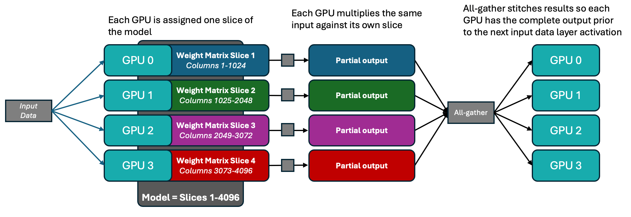
Each GPU multiplies the same input against its own 1024-wide slice, producing a 1024-wide partial output. None of them individually has the full 4096-wide result the next layer requires. All-gather stitches the four partial outputs back together into the complete 4096-wide result, and every GPU ends up with the full picture before the next layer can run.

This operation happens at essentially every layer boundary, for every single inference request, not just during training (the layer boundary is the transition point where local tensor shards are fully synchronized, recombined, or passed to subsequent operations). Serving a large model split across multiple GPUs looks, from the network’s perspective, like a miniature training job repeated on every forward pass, because every inference request triggers this split-compute-then-all-gather pattern, layer after layer, for the entire life of that request. So keep in mind that collective communications are not a training-only concern.

All-to-all: the pattern behind Mixture-of-Experts

All-to-all is the most network-intensive collective of all. Every GPU sends a distinct chunk of data to every other GPU simultaneously. This is not a fan-out or fan-in, but a full permutation.

This is central to Mixture-of-Experts (MoE) models, increasingly the architecture of choice for enterprises because they deliver more capability per active parameter than a dense model of equivalent size. In an MoE layer, a router (not talking network routers here) decides which “expert” sub-network each token should be processed by. Tokens then have to physically move to whichever GPU hosts their assigned expert, which is an all-to-all exchange. The tokens get processed, then get shuffled back to their original GPU with another all-to-all.

This happens on every forward pass. For an enterprise running MoE models in production, all-to-all is arguably the single most consequential collective to understand, even more so than all-reduce, because every MoE inference request generates this most expensive of all traffic patterns, making the network a critical medium at serving time as well as during training.

The parallelism strategy is fixed

The parallelism strategy (e.g., data-parallel, tensor-parallel, pipeline-parallel, expert-parallel), and how many GPUs are allocated to each, is typically a design decision made by ML engineers before a job launches, configured through the training or serving framework (Megatron-LM, DeepSpeed, PyTorch FSDP, vLLM, and similar). Auto-parallelism tools exist to search for a good configuration, but the chosen strategy is fixed for the duration of that job or deployment. It doesn’t change mid-run, and the network or scheduler has no role in deciding it on the fly.

The NCCL algorithm is dynamic

NCCL doesn’t use one algorithm for all-reduce regardless of size. NCCL dynamically chooses the algorithm based on message size, GPU node count, and detected topology:

• Ring algorithm: bandwidth-optimal, preferred for large messages, but latency scales with the number of participants (N-1 steps)
• Tree algorithm (binary or binomial): latency-optimal for small messages using fewer hops (log N steps), at some bandwidth cost
• Halving-doubling: efficient for power-of-2 GPU counts, used for reduce-scatter/all-gather phases

The algorithm choice determines whether the traffic pattern is sustained-and-sequential (ring: each link busy for a long, steady duration) or bursty-and-fan-shaped (tree: shorter bursts, more simultaneous small flows). This algorithm selection is mostly automatic, though it can be forced via environment variables (NCCL_ALGO, NCCL_PROTO) when debugging a performance problem or working around a topology quirk. From a network perspective, congestion management and buffer strategy will differ accordingly based on the traffic pattern, so understanding these different patterns is helpful when designing and troubleshooting AI data center networks.

Takeaways

1. Elephant flows in AI networks are the direct output of these specific, named operations. Knowing which collective produced a given flow tells you what shape to expect and what remediation makes sense.
2. Collective communication is a permanent fixture of large-model inference serving. All-gather driven by tensor parallelism keeps this traffic present throughout the life of a deployment, well past the end of training.
3. All-to-all is the pattern to design around first for any enterprise running Mixture-of-Experts models. It is structurally the most demanding traffic pattern on the fabric, and it recurs on every single request.
4. When troubleshooting a slow collective, remember the algorithm choice (ring vs. tree) is usually automatic, but it’s a legitimate, configurable lever, not a black box.

Next in this series: training vs. inference network requirements, revisited now with the vocabulary to go deep on why tensor-parallel and Mixture-of-Experts inference traffic deserves as much design attention as training traffic ever has.