Fabric Topologies for GPU Clusters

David Varnum

2 hours ago

Part 5 of a series on data center networking for AI

So far, we’ve covered the basics on GPU connectivity, collective communications, and training vs inference. We are now heading into territory more familiar to network engineers, and likely where most time will be spent doing network engineering for AI data centers.

The various networks that comprise an AI data center

In traditional data centers, there are typically just a couple of networks – data and management. The data serves north/south and east/west, with storage often riding on top of the same fabric.

In data centers that support AI clusters, several interconnected networks are often leveraged:

Back-end compute network – the dedicated fabric carrying only GPU-to-GPU collective traffic, as introduced in Part 1 of this series.
Front-end network – the north/south network that connects users, APIs, and services to the AI cluster
Storage network – storage connectivity for training data, checkpoints, and the KV cache tiering hierarchy from Part 4
Out-of-band management network – used for obvious reasons such as host management, control-plane services, and the Board Management Controllers (BMCs) for remote administration

In serious AI infrastructure builds, each of these networks have independent topology, oversubscription, and often independent switch vendor choices entirely. A back-end fabric’s latency and loss sensitivity generally rule out sharing it with general-purpose traffic. Smaller deployments sometimes consolidate front-end and storage together to save cost, but the back-end/GPU fabric essentially never gets folded in.

To visualize this from the perspective of an H100, the physical connectivity may look something like below, where the green lines are ConnectX ports connecting to the front-end fabric, the purple lines are OSFP ports connecting to the back-end fabric, and the BMC connected to the out-of-band network.

The remainder of this post primarily concerns the back-end network.

Clos/leaf-spine, quickly recapped

The folded-Clos (fat-tree) topology is built from identical switch building blocks arranged in tiers, with every leaf connected to every spine via equal-cost paths. Its defining property is you scale horizontally by adding spine switches, not by replacing existing hardware, and ECMP spreads load across the available equal-cost paths.

A folded-Clos AI fabric is the same topology as the leaf-spine fabric you’ve already designed for years. It’s the same mathematical structure Charles Clos originally described for telephone switching in 1953. What changes between an enterprise Clos and an AI Clos is entirely in provisioning and silicon, not the underlying math:

Oversubscription ratio – enterprise Clos commonly runs 3:1 or 4:1, whereas AI Clos is provisioned non-blocking, 1:1.
Silicon capabilities – AI-oriented ASICs add adaptive routing, RoCEv2-aware congestion control, and much deeper packet buffers tuned for incast and elephant flows, none of which a typical enterprise Clos switch needs.
Rail-alignment – the GPU-position-to-rail wiring pattern from Part 2 is a wiring convention layered on top of the same Clos structure, not a different topology.

This doesn’t require learning an entirely new discipline. It’s the Clos network you already operate, provisioned differently and built on silicon with AI-specific capabilities added.

Scaling the rail-optimized design beyond one pod

Quick refresher from Part 2: each GPU’s dedicated NIC lands on its own rail switch, and this wiring pattern repeats identically across every server, so any GPU in a given position is always exactly one hop from the same GPU position on any other server. At larger scale, that rail tier becomes the leaf tier of a Clos, with a spine tier connecting rails, and once a cluster exceeds what a single pod’s spine can address, a super-spine tier connects multiple pods together.

Two design details worth internalizing when it comes to pod scaling:

Switch radix determines pod size. A spine switch’s port count caps how many rail switches it can connect to at full non-blocking bandwidth. Current-generation high-radix switches (51.2Tbps-class ASICs, standard across networking vendors as you’ll see below) push single-pod scale well into the thousands of GPUs before a super-spine tier is needed at all. In reality, for most enterprise deployments, you will never need one.

Scale-up vs. scale-out is a critical distinction. NVLink/NVSwitch (Part 2) is “scale-up”, meaning it grows the GPU count reachable at full bandwidth without touching this Ethernet/InfiniBand fabric at all. Everything in this post is “scale-out”, meaning it only carries what NVLink couldn’t. To ask “why can’t we just add more GPUs to this node” is asking a scale-up question. To ask “why can’t we add more nodes” is asking a scale-out question.

The physical port math behind “non-blocking”

Earlier posts in this series drew rail-to-spine connectivity as a single logical line for clarity. In an actual build, that line represents many physical links, and the math behind it is worth discussing, because it’s what determines switch selection.

If a rail switch has 48 GPU-facing downlink ports at 400G each, maintaining a non-blocking fabric end to end requires 48×400G of aggregate uplink bandwidth leaving that switch. In practice, those uplinks are split across multiple spine switches, both to keep any single spine switch’s radix requirement reasonable and to provide redundancy against a spine switch failure.

Rather than matching port count 1:1 (48 downlinks, 48 uplinks), a common approach is to consolidate onto fewer, faster uplink ports (e.g., 48×400G downlinks paired with 24×800G uplinks). The aggregate bandwidth is identical (19.2Tbps in both directions), so the fabric remains fully non-blocking. This consolidation is common for good reasons:

fewer transceivers and cables at the more expensive, typically optical uplink tier
fewer ports consumed on each spine switch per leaf, which relaxes the switch radix constraint further
modern ASICs support flexible port breakout from the same SerDes lanes, so building a leaf with mixed downlink/uplink speeds off one piece of silicon is a standard configuration

However, there is one nuance worth flagging. Consolidating from 48 paths to 24 paths reduces ECMP entropy, meaning fewer independent paths leading to coarser granularity for hash-based load spreading, which in isolation makes elephant-flow hash collisions somewhat more consequential. This is why adaptive routing, covered next, matters more as designs consolidate onto fewer, faster links rather than less.

Adaptive routing: what it is, and where it lives

Before we get into adaptive routing, we first need to understand the constraints of L3 Equal-cost Multi-pathing (ECMP) and BGP. BGP, or whatever underlay protocol is in use, operates at the control plane. Its job is computing which next-hops are valid, equal-cost candidates to reach a given destination using network-layer reachability information. ECMP itself uses a 5-tuple to load balance flows between a source and destination where all packets of a single flow follow the same exact path for the life of the flow. In a network that is handling RDMA traffic, especially elephant flows transmitted at line-rate on RDMA-capable NICs, the single path limitation can quickly congest links and lead to degraded performance. The issue is compounded when multiple flows hash to the same link, which is common during collective operations like all-reduce.

Since ECMP does not adapt or reroute traffic, packets will buffer due to congestion when a single link is saturated. A single congested path can be catastrophic and costly, noticeably impacting user experience and the bottom line for the business. This is where adaptive routing comes in, aiming to improve traffic distribution in RoCEv2 networks.

Adaptive routing is a mechanism to dynamically route traffic based on link utilization and real-time network congestion, offering a much better distribution of traffic than the ECMP 5-tuple algorithm. Adaptive routing operates at the data plane, inside the switch ASIC, in real time. Given the candidate paths the control plane already computed, adaptive routing decides which one an actual packet or flow takes right now, based on live congestion signals (e.g., local queue depth, port utilization) that BGP has no visibility into and reconverges far too slowly to react to. BGP operates on the order of seconds whereas adaptive routing reacts on the order of microseconds. In other words, adaptive routing is a data-plane, switch-silicon function, not a control-plane (BGP) function.

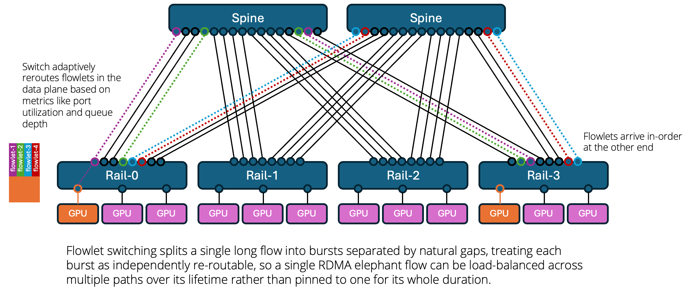
With adaptive routing, we have the flexibility of routing packets on a per-flowlet or per-packet basis.

A flowlet is a burst of packets from a single flow that’s separated from the next burst by a gap large enough to treat them as independent scheduling units for load balancing purposes. So instead of load-balancing at the flow level or the packet level, you load-balance at the sub-flow “burst” level. Flowlets are determined by the switch; the RDMA NICs are unaware. Packet ordering is preserved by the switching fabric while allowing for much better distribution of traffic.

Another option is per-packet load-balancing, also known as packet spraying, which provides maximum load distribution across the fabric at the risk of introducing out-of-order packets. To solve this, NVIDIA’s ConnectX and BlueField NICs do the reordering. The switch makes the adaptive routing decision per packet; packets arrive at the destination NIC likely out of order, and NVIDIA’s Direct Data Placement (DDP) on the BlueField-3 or ConnectX-8 SuperNIC re-orders those packets into the correct sequence in GPU memory before the application sees the data, making adaptive routing transparent. This is possible because RDMA writes carry explicit memory-offset placement info rather than being a pure ordered byte-stream, meaning the NIC can place arriving data correctly in memory even if it’s out of order, and only needs to handle completion/ordering semantics at the RDMA layer rather than the wire layer. This decouples correctness from strict packet order, letting the fabric use more aggressive adaptive routing/spraying than conservative flowlet gap thresholds would normally allow.

In summary:

Classic ECMP hashes an entire flow to one path for its whole lifetime.
Flowlet switching instead splits a single long flow into bursts separated by natural gaps, treating each burst as independently re-routable, so a single RDMA elephant flow can be load-balanced across multiple paths over its lifetime rather than pinned to one for its whole duration.
Packet spraying takes it a step further with per-packet load-balancing, relying on the receiving RDMA NIC itself to do the reordering.

Would you use one over the other, or both?

In practice it’s workload-dependent, and this is why vendors ship both as configurable modes rather than picking one:

Flowlet / conservative gap-threshold routing – better fit where you don’t have guaranteed end-to-end NIC-side reorder support, or where the workload is latency-sensitive per-message rather than throughput-maximizing (some storage-over-RDMA use cases, mixed RDMA/non-RDMA fabrics). Packet spraying – better fit for pure GPU-to-GPU collective operations (allreduce, alltoall) in AI training, which tolerate packet reordering and want maximum path utilization since job completion time is the dominant KPI, not per-packet latency.

Cisco’s own reference architecture reflects this explicitly – they support Dynamic Load Balancing with load and congestion awareness, weighted-cost multipath, per-packet and selective packet spray (for example RDMA vs. non-RDMA), and policy-based flowlet load balancing as selectable modes on the same silicon, often policy-differentiated by traffic type (DSCP/ACL-based selection).

Regarding configuration, the capability itself typically ships as a feature flag on modern AI-optimized ASICs. But turning it on effectively requires tuning underneath using mechanisms like DCQCN and ECN marking thresholds, PFC watermarks and watchdog timers, per-priority buffer allocation, and flowlet gap-timer thresholds. Poorly tuned PFC thresholds are a well-documented cause of head-of-line blocking and, in bad cases, PFC storms worse than not having lossless behavior at all. This is the territory I’ll cover in Part 7 (RDMA transport), so treat this section as the preview.

When Clos stops being the right answer

Clos is the correct default at essentially every scale you’ll encounter in enterprise practice. It’s worth understanding where it breaks down, because the alternative, Dragonfly, is an option that shows up in hyperscale training literature and increasingly in merchant silicon datasheets.

At extreme scale (e.g., tens of thousands of GPUs) a fully non-blocking Clos requires so many spine switches and so much cabling that cost and physical build complexity become the binding constraint, not bandwidth. Dragonfly’s answer is to organize switches into groups, fully connect switches within a group locally, and connect groups to each other directly via global links, rather than routing every inter-group hop through a dedicated spine tier.

Dragonfly needs fewer total switches and less cabling than an equivalent-scale Clos, at the cost of routing complexity, because global links aren’t uniform equal-cost paths the way Clos spine links are.

Dragonfly’s adaptive routing behavior

Dragonfly deliberately builds in path diversity through a minimal/non-minimal adaptive routing scheme. By default, traffic between two groups takes the direct global link connecting them with minimal routing. When that direct link is congested, the switch adaptively reroutes to non-minimal routing, sending traffic through a third, intermediate group instead, trading one extra hop for avoiding the congested link. The adaptive, congestion-aware behavior is the actual point of Dragonfly, not just the group structure.

The topology and physical links never change between these two scenarios – only the real-time routing decision does, made by the same data-plane adaptive routing mechanism described above, reacting to live congestion signals on the direct link.

The vendor landscape

This generation of AI-optimized, high-radix silicon is a cross-vendor phenomenon rather than one company’s exclusive advantage. This space is moving fast, so keep in mind the data below is just a point-in-time and not completely comprehensive:

NVIDIA – Spectrum-X (built on the Spectrum-4 ASIC, 51.2Tbps) is NVIDIA’s own Ethernet AI fabric line, paired with ConnectX NICs and BlueField DPUs as a tightly integrated, turnkey stack. NVIDIA also sells InfiniBand directly (Quantum-X800, built on the Quantum-3 ASIC) for customers who want InfiniBand’s native adaptive routing and lossless behavior rather than Ethernet.

Broadcom – sells merchant silicon rather than switches directly: Tomahawk 5, and the newer Tomahawk Ultra and Tomahawk 6, used by many other switch vendors as the silicon underneath their own platforms. Tomahawk 5 explicitly supports both Clos and non-Clos topologies, including torus, Dragonfly, Dragonfly+, and Megafly, alongside advanced adaptive routing and dynamic load balancing purpose-built for AI/ML traffic patterns.

Cisco – Silicon One G200 (51.2Tbps, 5nm) is Cisco’s answer, shipping in the Nexus 9364E-SG2, a 64-port 800GbE switch with 256MB of on-die packet buffer. Cisco has positioned this generation as Ultra Ethernet Consortium-aligned and has already announced a next-generation G300.

Arista – its Etherlink line is frequently cited as the leading non-NVIDIA answer for large-scale Ethernet AI fabrics. The 7800R4 AI spine supports 576 ports of 800GbE in a single chassis, and the 7700R4 Distributed Etherlink Switch scales to tens of thousands of accelerators in a single domain. Meta selected it for its Disaggregated Scheduled Fabric at roughly 100,000-accelerator scale.

Juniper – Juniper’s AI switches (the QFX5230/QFX5240 family) also run on Broadcom Tomahawk 5 silicon rather than a custom ASIC. Juniper’s real differentiation is Apstra, its intent-based fabric automation: an operator defines intent (e.g., a 32-node leaf-spine at 1:1 oversubscription, RoCEv2-ready) and Apstra generates the actual device configuration.

The throughline: 51.2Tbps-class silicon is now the common baseline across NVIDIA, Broadcom (and everyone building on it), and Cisco simultaneously, an industry-wide generational baseline with the next generation (Broadcom’s Tomahawk 6, at roughly double the bandwidth) already arriving.

Takeaways

Default to rail-optimized Clos for essentially every enterprise engagement – from tens of GPUs through several thousand in a single pod. It’s simpler to operate, uses well-understood ECMP as a foundation, and modern switch radix means a super-spine tier is rarely needed at all.
Dragonfly and its modern variants are a hyperscale training-cluster decision, relevant at tens of thousands of GPUs where cabling and switch count dominate cost.
Scale-up (NVLink) and scale-out (everything in this post) are separate strategies and conflating them is a reliable way to end up solving the wrong problem.
When a design consolidates onto fewer, faster uplinks to save cost, confirm the switch vendor’s adaptive routing and flowlet load-balancing options to best suit the expected traffic patterns. Reduced ECMP entropy makes this more important.
Non-blocking is a provisioning approach against assumed traffic patterns, and does not guarantee congestion won’t occur. You must size and monitor against realistic worst-case concurrent bursts, particularly in multi-tenant fabrics (Part 4).

Next in this series: the control plane – BGP EVPN/VXLAN for AI fabrics, and how the underlay we’ve assumed throughout this post is actually built and operated.

REFERENCES: